Representative Values of Hydraulic Properties

Aquifer tests (pumping tests, slug tests and constant-head tests) are performed to estimate site-specific values for the hydraulic properties of aquifers and aquitards. Under certain circumstances, however, site-specific hydraulic property data may not be available when needed. For example, reconnaissance studies or scoping calculations may require hydraulic property values before on-site investigations are performed.

The following sections present representative hydraulic property values reported in the literature for horizontal and vertical hydraulic conductivity, storativity, specific yield and porosity. Refer to these values if site-specific data are unavailable for your study or to check the results of field and laboratory tests conducted at an investigation site.

Try out the interactive calculators for estimating hydraulic conductivity from grain size, specific storage and storativity!

Hydraulic conductivity is a measure of a material's capacity to transmit water. It is defined as a constant of proportionality relating the specific discharge of a porous medium under a unit hydraulic gradient in Darcy's law:

$$\nu =-Ki$$

where $\nu$ is specific discharge [L/T], $K$ is hydraulic conductivity [L/T] and $i$ is hydraulic gradient [dimensionless]. Coefficient of permeability is another term for hydraulic conductivity.

Note that hydraulic conductivity, which is a function of water viscosity and density, is in a strict sense a function of water temperature; however, given the small range of temperature variation encountered in most groundwater systems, the temperature dependence of hydraulic conductivity is often neglected.

Transmissivity is the rate of flow under a unit hydraulic gradient through a unit width of aquifer of given saturated thickness. The transmissivity of an aquifer is related to its hydraulic conductivity as follows:

$$T=Kb$$

where $T$ is transmissivity [L²/T] and $b$ is aquifer thickness [L].

Representative Values

The following tables show representative values of hydraulic conductivity for various unconsolidated sedimentary materials, sedimentary rocks and crystalline rocks (from Domenico and Schwartz 1990):

Unconsolidated Sedimentary Materials
Material	Hydraulic Conductivity (m/sec)
Gravel	3×10-4 to 3×10-2
Coarse sand	9×10-7 to 6×10-3
Medium sand	9×10-7 to 5×10-4
Fine sand	2×10-7 to 2×10-4
Silt, loess	1×10-9 to 2×10-5
Till	1×10-12 to 2×10-6
Clay	1×10-11 to 4.7×10-9
Unweathered marine clay	8×10-13 to 2×10-9

Sedimentary Rocks
Rock Type	Hydraulic Conductivity (m/sec)
Karst and reef limestone	1×10-6 to 2×10-2
Limestone, dolomite	1×10-9 to 6×10-6
Sandstone	3×10-10 to 6×10-6
Siltstone	1×10-11 to 1.4×10-8
Salt	1×10-12 to 1×10-10
Anhydrite	4×10-13 to 2×10-8
Shale	1×10-13 to 2×10-9

Crystalline Rocks
Material	Hydraulic Conductivity (m/sec)
Permeable basalt	4×10-7 to 2×10-2
Fractured igneous and metamorphic rock	8×10-9 to 3×10-4
Weathered granite	3.3×10-6 to 5.2×10-5
Weathered gabbro	5.5×10-7 to 3.8×10-6
Basalt	2×10-11 to 4.2×10-7
Unfractured igneous and metamorphic rock	3×10-14 to 2×10-10

To Convert	Multiply By	To Obtain
m/sec	100	cm/sec
m/sec	2.12×106	gal/day/ft2
m/sec	3.2808	ft/sec

Grain Size Relationships

A number of empirical formulas, some dating back over a century, have been proposed which attempt to relate the hydraulic conductivity of an unconsolidated geologic material (granular sediment or soil) to its grain size distribution obtained from sieve analysis. While these formulas can be useful as a first approximation of $K$, one should bear in mind that their generality is limited by a number of factors including the following:

1. the number of sediment samples used to develop the formula
2. the geologic environment(s) comprising the samples used to develop the formula
3. the range of grain size assumed for the formula
4. the uniformity of grain size assumed for the formula

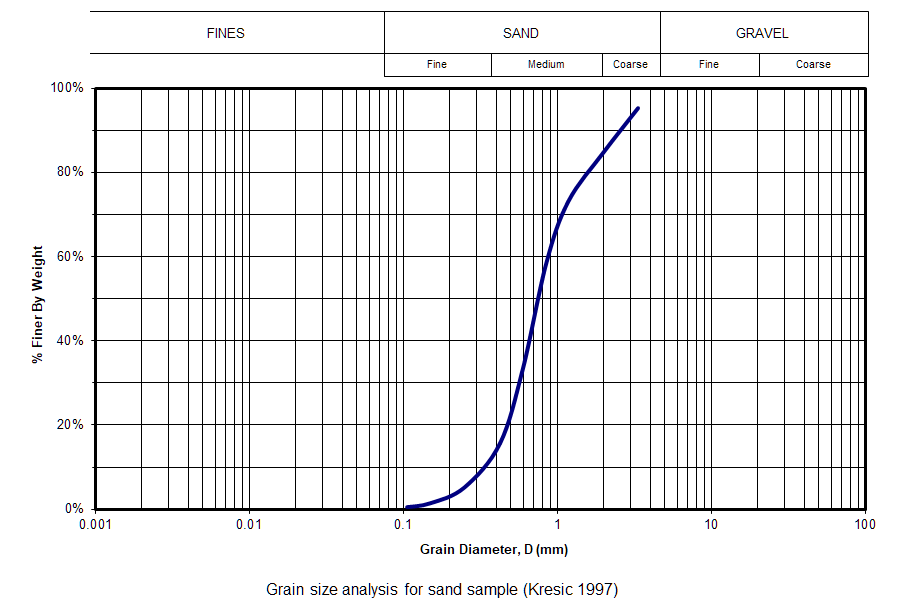
Equations for estimating $K$ from grain size commonly use two metrics from a grain size distribution plot: $D_{10}$, the grain diameter for which 10% of the sample is finer (90% is coarser), and $D_{60}$, the grain diameter for which 60% of the sample is finer (40% is coarser). $D_{10}$ is frequently taken as the effective diameter of the sample while the ratio $C_U$ = $D_{60}$/$D_{10}$ is known as the coefficient of uniformity.

The following calculator uses formulas by Hazen, Kozeny-Carmen, Beyer and Wang et al. to estimate $K$ from grain size and porosity data.

Data For Computing K From Grain Size Distribution
D10 =		mm
D60 =		mm
Total Porosity (n) =		[-]
Gravitational Acceleration (g) =		m/s²
Kinematic Viscosity (ν) =		m²/s
1 inch = 25.4 mm g = 9.8 m/s² ν = 1.2×10-6 m²/s at 13°C (55°F)

Hydraulic Conductivity (K) Estimated From Grain Size Data
D10 =		mm
D60 =		mm
CU =		[-]
n =		[-]
g =		m/s²
ν =		m²/s
Method	K (m/s)	K (cm/s)	K (ft/d)
Hazen1 (KH)
Kozeny-Carmen2 (KKC)
Beyer3 (KB)
Wang et al.4 (KW)
Average
Minimum
Maximum
Max/Min
10.1 mm ≤ D10 ≤ 3 mm; CU ≤ 5 2silts, sands and gravelly sands 30.06 mm ≤ D10 ≤ 0.6 mm; 1 ≤ CU ≤ 20 40.05 mm ≤ D10 ≤ 0.83 mm; 0.09 mm ≤ D60 ≤ 4.29 mm; 1.3 ≤ CU ≤ 18.3

Hazen Formula

Hazen (1892; 1911) developed a simple formula for estimating the hydraulic conductivity of a saturated sand from its grain size distribution:

$$K_H=C_H{D}_{10}^2$$

where $K_H$ is hydraulic conductivity [cm/s], $C_H$ is an empirical coefficient equal to 100 cm^‑1s^‑1 and $D_{10}$ is measured in cm.

As reported by Carrier (2003), $C_H$ is most commonly given as 100 but published values range over two orders of magnitude from 1 to 1000 cm^‑1s^‑1. The Hazen formula is assumed valid for 0.1 mm ≤ $D_{10}$ ≤ 3 mm and $C_U$ ≤ 5 (Kresic 1997).

Kozeny-Carmen Formula

An equation attributed to Kozeny and Carmen (Freeze and Cherry 1979; Rosas et al. 2014) may be used to estimate the hydraulic conductivity of sediments and soils:

$$K_{KC}=C_{KC}\frac{g}{\nu }\frac{n^3}{{\left(1-n\right)}^2}{D}_{10}^2$$

where $K_{\mathrm{KC}}$ is hydraulic conductivity [m/s], $C_{\mathrm{KC}}$ is an empirical coefficient equal to 1/180 [dimensionless], $g$ is gravitational acceleration [m/s²], $\nu$ is kinematic viscosity of water [m²/s] and $n$ is total porosity [dimensionless]. $D_{10}$ is measured in m.

The Kozeny-Carmen formula is assumed valid for sediments and soils composed of silt, sand and gravelly sand (Rosas et al. 2014).

Beyer Formula

Beyer (1964) also proposed a simple relationship for estimating hydraulic conductivity from a sediment's grain size distribution:

$$K_B=C_B\frac{g}{\nu }\text{ln}\left(\frac{500}{D_{60}/D_{10}}\right)D_{10}^2$$

where $K_B$ is hydraulic conductivity [m/s], $C_B$ is an empirical coefficient equal to 6×10^-4 [dimensionless], $g$ is gravitational acceleration [m/s²] and $\nu$ is kinematic viscosity of water [m²/s]. $D_{10}$ and $D_{60}$ are measured in m.

The Beyer formula is assumed valid for 0.06 mm ≤ $D_{10}$ ≤ 0.6 mm and 1 ≤ $C_U$ ≤ 20 (Kresic 1997).

Wang Et Al. Formula

Wang et al. (2017) developed another empirical formula for estimating hydraulic conductivity from the grain size distribution of a sediment or soil:

$$K_W=C_W\frac{g}{\nu }{\left(\log \frac{g{D}_{60}^3}{{\nu }^2}\right)}^{-1}{D}_{10}^2$$

where $K_W$ is hydraulic conductivity [m/s], $C_W$ is an empirical coefficient equal to 2.9×10^-3 [dimensionless], $g$ is gravitational acceleration [m/s²] and $\nu$ is kinematic viscosity of water [m²/s]. $D_{10}$ and $D_{60}$ are measured in m.

The Wang et al. formula is developed from a dataset (Rosas et al. 2014) characterized by 0.05 mm ≤ $D_{10}$ ≤ 0.83 mm, 0.09 mm ≤ $D_{60}$ ≤ 4.29 mm and 1.3 ≤ $C_U$ ≤ 18.3.

An anisotropy ratio relates hydraulic conductivities in different directions. For example, vertical-to-horizontal hydraulic conductivity anisotropy ratio is given by $K_z/K_r$ where $K_z$ is vertical hydraulic conductivity [L/T] and $K_r$ is radial (horizontal) hydraulic conductivity [L/T]. Anisotropy in a horizontal plane is given by $K_x/K_y$ where $K_x$ and $K_y$ are horizontal hydraulic conductivities in the $x$ and $y$ directions, respectively [L/T].

Todd (1980) reports values of $K_z/K_r$ ranging between 0.1 and 0.5 for alluvium and possibly as low as 0.01 when clay layers are present.

Representative Values

The following table shows representative values of horizontal and vertical hydraulic conductivities for selected rock types (from Domenico and Schwartz 1990):

Material	Horizontal Hydraulic Conductivity (m/sec)	Vertical Hydraulic Conductivity (m/sec)
Anhydrite	10-14 to 10-12	10-15 to 10-13
Chalk	10-10 to 10-8	5×10-11 to 5×10-9
Limestone, dolomite	10-9 to 10-7	5×10-10 to 5×10-8
Sandstone	5×10-13 to 10-10	2.5×10-13 to 5×10-11
Shale	10-14 to 10-12	10-15 to 10-13
Salt	10-14	10-14

Confined Aquifers

The storativity of a confined aquifer (or aquitard) is defined as the volume of water released from storage per unit surface area of the aquifer or aquitard per unit decline in hydraulic head. Storativity is also known by the terms coefficient of storage and storage coefficient.

Pumping a well in a confined aquifer releases water from aquifer storage by two mechanisms: compression of the aquifer and expansion of water.

In a confined aquifer (or aquitard), storativity is defined as

$$S=S_{s}b$$

where $S$ is storativity [dimensionless], $S_s$ is specific storage [L^-1] and $b$ is aquifer (or aquitard) thickness [L].

The typical storativity of a confined aquifer, which varies with specific storage and aquifer thickness, ranges from 5×10^-5 to 5×10^-3 (Todd 1980).

Specific storage is the volume of water that a unit volume of aquifer (or aquitard) releases from storage under a unit decline in head. Specific storage is related to the compressibilities of water and the aquifer (or aquitard) as follows:

$$S_s=\rho g\left(\alpha +n\beta \right)$$

where $\rho$ is mass density of water (= 1000 kg/m³) [M/L³], $g$ is gravitational acceleration (= 9.8 m/sec²) [L/T²], $\alpha$ is aquifer (or aquitard) compressibility [T²L/M], $n$ is total porosity [dimensionless], and $\beta$ is compressibility of water (= 4.4×10^-10 m sec²/kg or Pa^-1) [T²L/M].

Unconfined Aquifers

The storativity of an unconfined aquifer includes its specific yield or drainable porosity:

$$S=S_y+S_{s}b$$

where $S_y$ is specific yield [dimensionless].

Lowering of the water table in an unconfined aquifer leads to the release of water stored in interstitial openings by gravity drainage.

Compared to gravity drainage, aquifer compression and water expansion in a water-table aquifer yield relatively little water from storage; hence, $S_y\gg S_{s}b$ and $S\cong S_y$ in unconfined aquifers.

Storativity in unconfined aquifers typically ranges from 0.1 to 0.3 (Lohman 1972).

Representative Values

The following table provides representative values of specific storage for various geologic materials (Domenico and Mifflin [1965] as reported in Batu [1998]):

Material	Ss (ft-1)
Plastic clay	7.8×10-4 to 6.2×10-3
Stiff clay	3.9×10-4 to 7.8×10-4
Medium hard clay	2.8×10-4 to 3.9×10-4
Loose sand	1.5×10-4 to 3.1×10-4
Dense sand	3.9×10-5 to 6.2×10-5
Dense sandy gravel	1.5×10-5 to 3.1×10-5
Rock, fissured	1×10-6 to 2.1×10-5
Rock, sound	< 1×10-6

To Convert	Divide By	To Obtain
ft-1	0.3048	m-1

Freeze and Cherry (1979) provided the following compressibility values for various aquifer materials:

Material	Compressibility, α (m2/N or Pa-1)
Clay	10-8 to 10-6
Sand	10-9 to 10-7
Gravel	10-10 to 10-8
Jointed rock	10-10 to 10-8
Sound rock	10-11 to 10-9

Pa^-1 = m²/N = m sec²/kg

Specific Storage Calculator

$$S_s=\rho g\left(\alpha +n\beta \right)$$

Enter values for aquifer compressibility and porosity to compute specific storage.

Compute Specific Storage
Aquifer Compressibility (α) =		m²/N
Total Porosity (n) =		dimensionless
Density of Water (ρ) =		kg/m³
Gravitational Acceleration (g) =		m/sec²
Water Compressibility (β) =		m²/N
Specific Storage (Ss) =		m-1

Storativity Calculator

$$S=S_{s}b=\rho g\left(\alpha +n\beta \right)b$$

Enter values for aquifer compressibility, porosity and thickness to compute storativity.

Compute Storativity
Aquifer Compressibility (α) =		m²/N
Total Porosity (n) =		dimensionless
Aquifer Thickness (b) =		m
Density of Water (ρ) =		kg/m³
Gravitational Acceleration (g) =		m/sec²
Water Compressibility (β) =		m²/N
Storativity (S) =		dimensionless

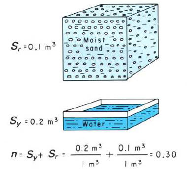
Specific yield is defined as the volume of water released from storage by an unconfined aquifer per unit surface area of aquifer per unit decline of the water table.

Bear (1979) relates specific yield to total porosity as follows:

$$n=S_y+S_r$$

where $n$ is total porosity [dimensionless], $S_y$ is specific yield [dimensionless] and $S_r$ is specific retention [dimensionless], the amount of water retained by capillary forces during gravity drainage of an unconfined aquifer. Thus, specific yield, which is sometimes called effective porosity, is less than the total porosity of an unconfined aquifer (Bear 1979).

Representative Values

Heath (1983) reports the following values (in percent by volume) for porosity, specific yield and specific retention:

Material	Porosity (%)	Specific Yield (%)	Specific Retention (%)
Soil	55	40	15
Clay	50	2	48
Sand	25	22	3
Gravel	20	19	1
Limestone	20	18	2
Sandstone (unconsolidated)	11	6	5
Granite	0.1	0.09	0.01
Basalt (young)	11	8	3

The following table shows representative values of specific yield for various geologic materials (from Morris and Johnson 1967):

Material	Specific Yield (%)
Gravel, coarse	21
Gravel, medium	24
Gravel, fine	28
Sand, coarse	30
Sand, medium	32
Sand, fine	33
Silt	20
Clay	6
Sandstone, fine grained	21
Sandstone, medium grained	27
Limestone	14
Dune sand	38
Loess	18
Peat	44
Schist	26
Siltstone	12
Till, predominantly silt	6
Till, predominantly sand	16
Till, predominantly gravel	16
Tuff	21

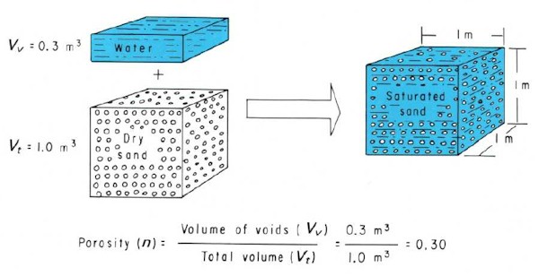
Porosity is defined as the void space of a rock or unconsolidated material:

$$n=V_v/V_t$$

where $n$ is porosity [dimensionless], $V_v$ is void volume [L³] and $V_t$ is total volume [L³].

Representative Values

The following tables show representative porosity values for various unconsolidated sedimentary materials, sedimentary rocks and crystalline rocks (from Morris and Johnson 1967):

Unconsolidated Sedimentary Materials
Material	Porosity (%)
Gravel, coarse	24 - 37
Gravel, medium	24 - 44
Gravel, fine	25 - 39
Sand, coarse	31 - 46
Sand, medium	29 - 49
Sand, fine	26 - 53
Silt	34 - 61
Clay	34 - 57

Sedimentary Rocks
Rock Type	Porosity (%)
Sandstone	14 - 49
Siltstone	21 - 41
Claystone	41 - 45
Shale	1 - 10
Limestone	7 - 56
Dolomite	19 - 33

Crystalline Rocks
Rock Type	Porosity (%)
Basalt	3 - 35
Weathered granite	34 - 57
Weathered gabbro	42 - 45

See also: Argonne National Laboratory, Wolff (1982)