Knowledge Base
Welcome to the AQTESOLV Knowledge Base! Find tips and answers to common questions relating to AQTESOLV, the world's leading software for the analysis of aquifer tests, from HydroSOLVE, Inc.
- Remember to click the Help buttons (or press F1) to get context-sensitive help in the AQTESOLV software.
- Choose Help>Contents and Index to access the Help file and look in the Q&A topic of the Support chapter to find answers to other common questions (v4.0+).
The following FAQ provides answers to frequently asked questions (v4.0+). Bookmark or print this page for future reference.
Aquifer Data
I don't know the thickness of my aquifer from well logs. What should I enter for aquifer thickness?
You'll have to estimate the thickness from other sources (published reports, geologic maps, geophysics, etc.). Another strategy is to perform a sensitivity analysis for a range of aquifer thickness values and see how changing the aquifer thickness affects your results.
What do I enter for the vertical-to-horizontal hydraulic conductivity ratio?
The default value is 1 (isotropic). For some aquifers (e.g., stratified aquifers), the value may be less than 1. If you have an independent estimate, you may enter it.
Wells
How do I edit wells in my data set?
Choose Edit>Wells, select a well in the list and click Modify to edit a well in an existing data set.
How do I add more wells to my data set?
Choose Edit>Wells>New to add pumping or observation wells to an existing data set.
How should I enter well coordinates?
Use any appropriate X,Y coordinate system (e.g., site coordinates) to enter well coordinates. Using X and Y coordinates (as opposed to radial distances) is essential when you are analyzing a pumping test with more than one pumping well or aquifer boundaries.
For simple cases, such as a pumping test in an infinite, isotropic aquifer with only one pumping well, you may enter 0,0 for the coordinates of the test well and R,0 for the observation wells where R is radial distance from the pumping well to the observation well.
Choose Edit>Wells>Modify to edit well coordinates.
Well Construction
How do I enter well screen depths?
Enter depths measured from the top of the aquifer not from land surface. In a confined aquifer, measure depths from the upper confining unit. In an unconfined aquifer, measure depths from the static water table. For a well screened across the water table, click here.
My well is screened across the water table. What do I enter for d (depth to top of screen) and L (screen length)?
For a well screened across the water table, enter d=0. Enter the submerged length of screen for L. Ignore any portion of the screen above the water table.
What is the casing radius?
The casing radius refers to the radius of the unperforated portion of the well pipe above the open interval (screen). The casing radius may be less than, equal to or greater than the well radius depending on the construction of your well.
What do I enter for the equipment radius?
Enter the effective radius of downhole equipment (e.g., pumping discharge line, transducer cable, etc.). When you enter the equipment radius greater than zero, AQTESOLV corrects the casing radius to account for the reduced area inside the casing. The equipment radius should be less than the casing radius. Enter zero for no correction.
What do I enter for the packer radius?
The packer radius only applies to certain solutions such as the McElwee-Zenner slug test model. Enter zero otherwise.
What do I enter for the well radius?
For a well without a filter pack, enter the screen radius or the wellbore radius for an open hole. For a well with a filter pack, enter the wellbore radius if the filter pack material is much more permeable than the formation; otherwise enter the screen radius. The well radius may be smaller than, equal to or larger than the casing radius depending on the construction of your well.
What do I enter for the skin radius?
Enter the skin radius greater than or equal to the well radius. Note that the skin radius only applies to certain solutions such as the KGS Model for slug tests.
When should I correct for filter pack porosity?
The optional correction for gravel pack porosity recommended by Bouwer and Rice (1976) is only required for slug tests when the well is screened across the water table. Do not apply the filter pack correction when the screen is fully submerged or when the aquifer is confined.
Pumping Rates
How do I enter the pumping rate for a constant-rate pumping test?
When you enter rates into AQTESOLV, enter the time for each measured rate as the elapsed time since the start of the test when the rate becomes active. Thus, for a constant-rate test, enter zero for time and the constant rate into the rates spreadsheet. You only need to enter one pumping rate for a constant-rate test.
For example, if you are analyzing drawdown data from a pumping test performed at a constant-rate of 100 gpm, you only need to enter the following row in the rates spreadsheet for the pumping well:
Tip: There is no need to enter a pumping rate corresponding to each drawdown measurement you collect.
How do I enter variable rates for a pumping test?
To edit rates for a pumping well, choose Edit>Wells>Modify.
In the Rates tab for the well, enter a time and rate for each change in rate. Time is elapsed time since the start of the test when each rate becomes active. Each rate that you enter represents a step change in the pumping rate during the test. Add rows to the spreadsheet as needed to accommodate the rate variations during your test.
For example, consider a step-drawdown test performed at rates of 50, 100 and 150 gpm with each step lasting 60 minutes. You would enter the following three rows into the rates spreadsheet for the pumping well:
How do I enter pumping rates for a test with recovery?
When you enter rates into AQTESOLV for a recovery test, first enter all of the rates measured prior to recovery. Then enter the time when recovery begins (enter this time as elapsed time since pumping began) and a rate of zero.
For example, if you are analyzing recovery data following a pumping test performed at a constant rate of 100 gpm for one day (1440 minutes), you need to enter the following two rows in the rates spreadsheet for the pumping well:
Tip: You can enter both drawdown and recovery data in the same AQTESOLV data set and analyze them together or separately.
Single-Well Tests/Step-Drawdown Tests
Do I need to enter both a pumping well and an observation well for a single-well test?
In AQTESOLV v4.0 and higher, you may enter pumping rates and observations into one well for a single-well pumping test (e.g., a step-drawdown test).
Use the Pumping Test Wizard (File>New) to create a new data set for single-well pumping test or choose Edit>Wells to edit data you've already entered.
Can I estimate S (storage coefficient) from a single-well test?
Estimation of S (storage coefficient) from a single-well test is dependent on the effective radius of the well/wellbore skin and turbulent well loss. Given these uncertainties, estimation of S from a single-well test is unreliable; however, a physically implausible estimate of S determined from a single-well test (e.g., S < 1x10⁻¹⁰) is a strong indicator of well inefficiency. In these instances, one may assign a realistic value of S and estimate wellbore skin factor from a single-well test.
Slug Tests
Why does a plot of my slug test data show displacement increasing with time?
It's likely that you need to transform the water-level data that you entered into AQTESOLV to displacement values. Displacement is the change in water level from its static (pre-test) level. When entered properly, displacement data from a slug test should be decreasing over time.
If you used a transducer to collect level data during your slug test, the data logger often records the height of the water column above the sensor. In a rising-head slug test, these untransformed data logger readings have an increasing trend over time. To transform the data logger measurements to displacement, subtract the static (pre-test) sensor reading from all of the level readings recorded during the test. After this transformation, the displacement data should decrease with time and approach zero as the water level in the well recovers to its pre-test position.
For more in-depth information, see our example on converting data logger measurements to displacement.
How do I transform/format data for a rising-head slug test?
See Why does a plot of my slug test data show displacement increasing with time? above.
Data Loggers/Importing Data
How do I configure Win-Situ 5 to work with AQTESOLV?
- Download and install the latest Win-Situ software for the Level TROLL from the In-Situ web site.
- Start the Win-Situ application.
- Choose General Settings from the Preferences menu.
- In the Time Format group of settings, select the Custom option and enter H:mm:ss in the Time input box (note the capital "H" in the format string configures a 24-hour clock for the time stamp).
- Click OK to save the new settings.
How do I convert logger data from linear sampling to a logarithmic schedule?
- Choose Edit>Wells, select a well and click Modify.
- Click the Observations tab.
- Click Select All to filter all observations.
- Click Filters to view filter options.
- In the Time Filters, check the option for Retain change in log time >= minimum and enter a value of 0.05 (=1/20) to retain 20 measurements per log cycle time. To retain 10 data points per log cycle time, enter 0.10 (=1/10). Click OK.
- Click OK to proceed with the filtering operation.
- AQTESOLV displays the number of observations filtered and the number of observations retained. Click OK.
Plots
How do I place the origin in the upper left corner of my plots?
Choose Format from the View menu and click the Graph tab to change the origin of the plot to the upper-left corner.
Why don't I see any data when I try to view an Agarwal plot?
To use an Agarwal plot to analyze data from a recovery test, make sure that your observation well data include a drawdown value measured at time tp when the pump was shut off.
Let us suppose that you pump a well for 1440 minutes and monitor recovery after turning off the pump. Your observation data must include a drawdown measurement at 1440 minutes (tp) if you intend to use the Agarwal method.
Why can't I choose the Distance-Drawdown plot option?
A graph of distance-drawdown (View>Distance-Drawdown) shows drawdown as a function of radial distance from a single pumping well. If you have more than one pumping well in your data set, you won't be able to choose the option for a Distance-Drawdown plot.
Curve Matching
Why does my plot of slug test data appear to show two straight lines?
The so-called double straight-line effect often occurs in wells screened across the water table due to drainage of the filter pack. Learn more…
My slug test data have a concave upward appearance. Where should I match my straight line?
Butler (1998) provides recommended head ranges to assist you in matching straight-line solutions (e.g., Bouwer and Rice [1976]) when data curvature makes a match ambiguous. In AQTESOLV, choose View>Options to activate the recommended head ranges which appear as two horizontal dashed lines on your data plot. Match the solution to the data within the recommended range. Learn more…
How can I tell if a match with the Cooper and Jacob (1946) straight-line method is valid?
In AQTESOLV, you have two options for checking when the Cooper and Jacob solution is valid:
- Choose View>Options>Plots tab and check the option to display Valid time for Cooper-Jacob approximation.
In the Valid Time tab, you may assign the critical value of u (default = 0.01).
AQTESOLV displays a vertical dashed line on your data plot to indicate the time when the Cooper and Jacob solution is valid. Note that the position of the line depends on the values of T (transmissivity) and S (storage coefficient) for the line that you've matched.
- In the Pro version of AQTESOLV, you may use derivative analysis (View>Options) to identify when the drawdown data have a constant slope on a semilog plot. A derivative plateau (= constant slope) indicates a period where you could match the Cooper-Jacob solution and estimate T of the aquifer assuming the underlying assumptions of the solution, such as infinite-acting aquifer conditions, are met.
How do I edit aquifer property values?
Choose Match>Toolbox. In the Parameters tab, enter new aquifer property values. Click Apply to see the effect of your changes.
Why don't I see a type curve displayed with my data?
- Correct any errors in your data set (View>Error Log).
- Choose a solution method (Match>Solution).
- Choose an appropriate plot type (not a diagnostic plot) from the View menu.
- Enable type curve display (View>Options).
- Expand range of axes in case type curve lies outside plot area (View>Format).
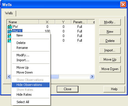
How do I hide/show well data for visual curve matching?
- View the list of wells in your data set (Edit>Wells).
- Right click over a well in the list and choose Hide Observations to hide the display of observation data for the well.
- Right click over a well in the list and choose Show Observations to show observation data for the well.
Printing
How do I fit the legend of my plot on a single page?
To fit more legend information on one page when printing a plot, change formatting options (View>Format>Legend tab) such as the font size or the number of items displayed.
Can I create a PDF of my plot using AQTESOLV?
If you have PDF (portable document format) software installed on your computer, you can print an AQTESOLV plot or report to a PDF. Choose File>Print and select the printer option that generates a PDF file.
Exporting Data
How do I export the derivative curve(s) to a file?
Choose the View>Derivative-Time. Choose File>Export and select Type Curve from the list of export options.
Error Messages
What should I do when I see "Check Errors" at the bottom of the AQTESOLV window?
When you see Check Errors on the status bar, choose View>Error Log to identify and correct errors that AQTESOLV has detected in your data set.
How do I correct errors listed in the Error Log?
Choose options from the Edit menu to modify the data set.
Why does the Error Log tell me there are no observations in my data set when I'm performing a forward solution?
This error only applies to curve matching analyses. You may ignore the message and proceed with a forward solution analysis.
Why does the Error Log tell me that the depth to the bottom of a well screen exceeds the aquifer thickness?
You are required to enter d (the depth to the top of the well screen) and L (screen length) for partially penetrating wells. The sum of d+L should not exceed the thickness of the aquifer. For more information on entering well depths, click here.
Why does the Error Log tell me maximum displacement is greater than initial displacement?
When you perform a slug test, the first reading (initial displacement) should be the maximum displacement during the test. If the Error Log displays the warning Maximum Displacement > Initial Displacement, AQTESOLV has detected one or more displacement data that exceed the initial displacement.
Choose Edit>Wells>Modify. The displacement data in the Observations tab should be less than or equal to the initial displacement found in the General tab for your test well.
Noise introduced during the initiation of a test (e.g., a solid slug impacting the water surface) can result in a maximum displacement that occurs after the start of the test and you may choose to ignore the warning in the Error Log.
Examples and tutorials are also available to help you with various topics!
FAQ for v3.x and older